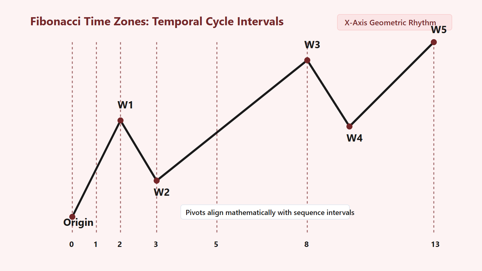
While most structural analysis focuses heavily on price geometry—measuring vertical distance and horizontal pullbacks—I never ignore the X-axis of my charts. The geometric structures formed by mass human psychology do not just expand in price; they evolve through time. To measure this, I apply Fibonacci Time Zones. Just as the Golden Ratio (1.618) governs the expansion of motive waves, the Fibonacci sequence (1, 2, 3, 5, 8, 13, 21, 34…) governs the temporal rhythm of market cycles. When I anchor a Fibonacci time measurement to a major structural extreme, I am looking for future inflection points where geometric exhaustion is highly probable.

The Temporal Dimension of Wave Mechanics

When analysts evaluate Elliott Wave structures, their immediate instinct is almost always confined to the vertical dimension: how many price units an impulse covers, the exact Fibonacci retracement depth of Wave 2, or the percentage extension reached by Wave 3. Yet price without time is an incomplete equation. The underlying engine driving market geometry is human sentiment, and collective sentiment does not operate purely as instantaneous reactions to external events. Mass psychology expands, consolidates, and reaches exhaustion along harmonic temporal cadences.

In my analytical practice, I treat time as the co-equal partner of price. A structural impulse pattern that advances 500 points over five periods possesses an entirely different mathematical signature than one covering identical distance over fifty periods. When I plot Fibonacci Time Zones across a chart, I establish a coordinate grid that tracks the structural tempo of the trend. These time zones are vertical intervals placed at distances corresponding to the sequence 1, 2, 3, 5, 8, 13, 21, 34, 55, 89, and beyond, measured from a foundational anchor point.

The beauty of this temporal progression lies in its exponential expansion. In the early stages of a nascent structural cycle, time markers sit tightly clustered together, reflecting rapid shifts in early directional momentum. As the cycle matures and transitions from explosive expansion into steady structural development, the intervals between projected inflection zones widen proportionally. This widening mirrors the natural deceleration of structural inertia as the macro wave approaches cyclical maturity.

Selecting the True Geometric Anchor Point

The precision of any Fibonacci time calculation depends entirely on where the initial anchor is placed. A common analytical mistake is arbitrary anchor selection—choosing a minor swing high or low simply because it appears visually prominent on an intraday timeframe. In my work, I anchor time projections strictly to verified structural extremes that denote the absolute termination of an entire wave degree.

When establishing an initial time zone grid, I isolate two primary structural junctures:

• The Origin of the Primary Motive Sequence: The terminal low of an antecedent multi-wave correction (the major Wave (C) or Wave (2) low) serves as the zero coordinate. This point marks the birth of new structural momentum.
• The Apex of Wave 1 or Wave A: The first major counter-directional pivot establishes the fundamental cycle baseline. The temporal distance between Coordinate 0 (the cycle origin) and Coordinate 1 (the termination of the first sub-wave) establishes the unit time period (T) that scales all subsequent intervals.

Once this foundational baseline distance is fixed, every subsequent vertical line marks an integer multiple of the base duration scaled by the Fibonacci sequence. The subsequent markers do not forecast whether the market must establish a crest or a trough at that exact timestamp; rather, they mark temporal thresholds where the reigning geometric vector is mathematically prone to directional transition.

Spatial-Temporal Confluence: Where Price Meets Time

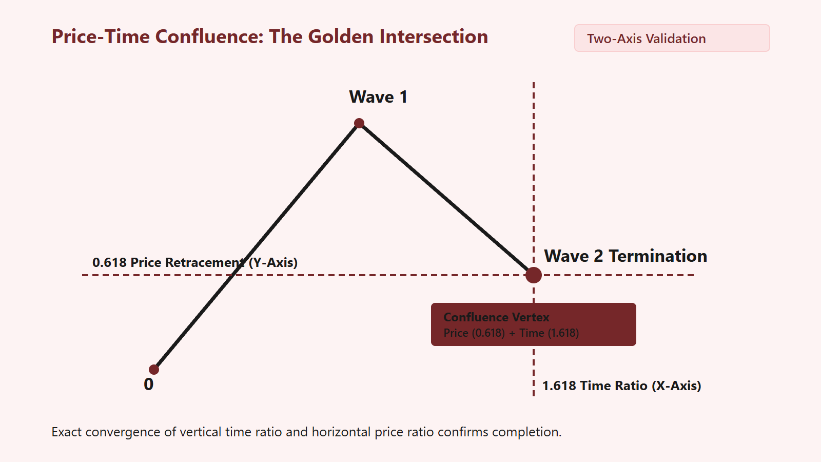
Isolated indicators possess limited predictive utility. The true power of Fibonacci Time Zones emerges when I observe spatial-temporal confluence—the precise intersection of a vertical Fibonacci price projection and a horizontal Fibonacci time interval. I refer to these coordinates as Geometric Nexus Points.

Consider a market advancing within an extended third wave. Through price geometry, I determine that Wave 3 reaches its optimal 1.618 expansion relative to Wave 1 at a specific structural coordinate. Simultaneously, my temporal sequence indicates that the 34th time unit intersects that exact same zone within a narrow window. When price reaches its quantitative Fibonacci objective at the exact moment the temporal sequence completes its cycle interval, the probability of structural exhaustion increases dramatically.

I observe that when price reaches a Fibonacci target ahead of its scheduled temporal window, the structure rarely initiates a full trend reversal immediately. Instead, the market frequently enters a protracted, sideways consolidation (such as a complex Flat or Triangle) to “consume time” until the corresponding Fibonacci time boundary is reached. Conversely, if the temporal boundary arrives before price has fulfilled its minimum geometric requirements, the prevailing impulse frequently accelerates in a violent blow-off move to bridge the remaining spatial gap.

Temporal Ratios in Corrective Consolidations

Corrective structures are notoriously time-consuming, often occupying between 61.8% and 161.8% of the total elapsed time of the preceding motive wave. When I track complex sideways corrections such as Expanded Flats, Triangles, or Double Combinations, Fibonacci time intervals provide the discipline required to avoid premature directional commitments.

During prolonged consolidations, market participants consistently suffer from psychological fatigue. They mistake minor intraday swings for the resumption of the macro trend, only to be repeatedly whipsawed as the sideways pattern persists. By calculating the elapsed duration of prior impulse legs and projecting the 0.618, 1.000, and 1.618 time extensions into the future, I can anticipate precisely how long the corrective phase must churn before the structural geometry achieves mathematical balance.

Key temporal relationships I routinely quantify include:

• Wave 2 vs. Wave 1 Duration: Wave 2 pullbacks frequently consume between 0.618 and 1.382 of the time required to construct Wave 1.
• Wave 4 Duration Symmetry: When Wave 2 is sharp and brief (consuming minimal time), Wave 4 almost universally expands into a prolonged sideways structure, consuming 1.618 to 2.618 times the duration of Wave 2 in accordance with the Guideline of Alternation.
• Corrective Leg Equality: In a standard A-B-C zigzag, Wave C typically requires an elapsed duration equal to Wave A (1.000 ratio), or expands to 1.618 of Wave A’s duration when unfolding as an elongated impulse.

Methodology: Step-by-Step Implementation of Time Projections

To implement this methodology systematically across your structural charting, follow these precise analytical protocols:

1. Identify the Macro Structural Anchor: Locate the unequivocal termination of the previous major trend degree. Verify that this extreme cannot be subdivided into remaining unfinished sub-waves.
2. Determine the Initial Unit Interval: Measure the chronological span between the anchor origin and the crest of the first impulsive subdivision. This forms the baseline unit interval.
3. Project the Time Progression: Project the sequence markers (1, 2, 3, 5, 8, 13, 21, 34, 55, 89…) along the time axis. Highlight zones where multi-degree time projections overlap, creating “time clusters.”
4. Map Price Retracements and Extensions: Overlay standard Fibonacci price tools (retracements and trend-based extensions) to identify the spatial coordinates that align with major wave targets.
5. Monitor Price Behavior at the Intersection: As price approaches the designated spatial-temporal nexus, examine the internal sub-wave structure. Look for terminal patterns such as ending diagonals, momentum divergence, or complete 5-wave micro-sequences.

By treating time not as an arbitrary backdrop but as a dynamic mathematical dimension, I eliminate the guesswork associated with standard pattern recognition. Market cycles are rhythmic, fractal, and governed by harmonious geometric laws. When you synchronize your analysis with the temporal rhythm of the Fibonacci sequence, you unlock an entirely new tier of structural clarity.